Welcome to the first part in this tutorial series introducing AI (machine learning) for medicine! These tutorials were initially made to go along with the the AI in Medicine workshop series, hosted by UBC and Queens medical school, so feel free to check out the companion slides and videos here.
Throughout these tutorials, we will use the Python programming language and I recommend completing these projects in ‘Google Colaboratory’ notebooks. With Google Colab, you can program and apply machine learning concepts directly in your browser interactively, without having to download and install anything.
Table of Contents:
- 1. Importing relevant libraries/modules
- 2. Loading the Breast Cancer Dataset
- 3. Converting to a dataframe and exploring the dataset
- 4. Basic Analysis
- 5. More Complex Analysis
1. Importing relevant libraries/modules
The first steps in almost any programming analysis is to load any relevant packages that you will need. In Python, these are known as modules or libraries, and are loaded through using the import and from commands.
For our introduction to scientific programming, we will use the following libraries:
Pandasfor creating and analyzing dataframes, which are like Excel tablesScipyandnumpyfor doing mathematical analysis on the datamatplotlib.pyplotfor creating and viewing plotssklearn(Scikit-learn) for accessing the breast cancer dataset
You can see below we use the as command so we can more conveniently refer to the libraries by shorter names like pd, np, and plt
import pandas as pd
import scipy
import numpy as np
import matplotlib.pyplot as plt
from sklearn.datasets import load_breast_cancer
2. Loading the Breast Cancer Dataset
We will load the Wisconsin Breast Cancer Dataset, view the data, visualize some plots and do some basic analysis.
# This is a comment. Everything preceded by a '#' is a comment and will not be run as code.
# Tip: you can use Ctrl+Enter to run a code cell, or Shift+Enter to run a code cell and proceed to the next one automatically

#Let's load the breast cancer dataset into a variable called dataset:
dataset = load_breast_cancer()

#Everything that is  held in the dataset variable can be viewed by using the print command. But this is not easy to understand.
print(dataset)
{'data': array([[1.799e+01, 1.038e+01, 1.228e+02, ..., 2.654e-01, 4.601e-01,
        1.189e-01],
       [2.057e+01, 1.777e+01, 1.329e+02, ..., 1.860e-01, 2.750e-01,
        8.902e-02],
       [1.969e+01, 2.125e+01, 1.300e+02, ..., 2.430e-01, 3.613e-01,
        8.758e-02],
       ...,
       [1.660e+01, 2.808e+01, 1.083e+02, ..., 1.418e-01, 2.218e-01,
        7.820e-02],
       [2.060e+01, 2.933e+01, 1.401e+02, ..., 2.650e-01, 4.087e-01,
        1.240e-01],
       [7.760e+00, 2.454e+01, 4.792e+01, ..., 0.000e+00, 2.871e-01,
        7.039e-02]]), 'target': array([0, 0, 0, 0, 0, 0, 0, 0, 0, 0, 0, 0, 0, 0, 0, 0, 0, 0, 0, 1, 1, 1,
       0, 0, 0, 0, 0, 0, 0, 0, 0, 0, 0, 0, 0, 0, 0, 1, 0, 0, 0, 0, 0, 0,
       0, 0, 1, 0, 1, 1, 1, 1, 1, 0, 0, 1, 0, 0, 1, 1, 1, 1, 0, 1, 0, 0,
       1, 1, 1, 1, 0, 1, 0, 0, 1, 0, 1, 0, 0, 1, 1, 1, 0, 0, 1, 0, 0, 0,
       1, 1, 1, 0, 1, 1, 0, 0, 1, 1, 1, 0, 0, 1, 1, 1, 1, 0, 1, 1, 0, 1,
       1, 1, 1, 1, 1, 1, 1, 0, 0, 0, 1, 0, 0, 1, 1, 1, 0, 0, 1, 0, 1, 0,
       0, 1, 0, 0, 1, 1, 0, 1, 1, 0, 1, 1, 1, 1, 0, 1, 1, 1, 1, 1, 1, 1,
       1, 1, 0, 1, 1, 1, 1, 0, 0, 1, 0, 1, 1, 0, 0, 1, 1, 0, 0, 1, 1, 1,
       1, 0, 1, 1, 0, 0, 0, 1, 0, 1, 0, 1, 1, 1, 0, 1, 1, 0, 0, 1, 0, 0,
       0, 0, 1, 0, 0, 0, 1, 0, 1, 0, 1, 1, 0, 1, 0, 0, 0, 0, 1, 1, 0, 0,
       1, 1, 1, 0, 1, 1, 1, 1, 1, 0, 0, 1, 1, 0, 1, 1, 0, 0, 1, 0, 1, 1,
       1, 1, 0, 1, 1, 1, 1, 1, 0, 1, 0, 0, 0, 0, 0, 0, 0, 0, 0, 0, 0, 0,
       0, 0, 1, 1, 1, 1, 1, 1, 0, 1, 0, 1, 1, 0, 1, 1, 0, 1, 0, 0, 1, 1,
       1, 1, 1, 1, 1, 1, 1, 1, 1, 1, 1, 0, 1, 1, 0, 1, 0, 1, 1, 1, 1, 1,
       1, 1, 1, 1, 1, 1, 1, 1, 1, 0, 1, 1, 1, 0, 1, 0, 1, 1, 1, 1, 0, 0,
       0, 1, 1, 1, 1, 0, 1, 0, 1, 0, 1, 1, 1, 0, 1, 1, 1, 1, 1, 1, 1, 0,
       0, 0, 1, 1, 1, 1, 1, 1, 1, 1, 1, 1, 1, 0, 0, 1, 0, 0, 0, 1, 0, 0,
       1, 1, 1, 1, 1, 0, 1, 1, 1, 1, 1, 0, 1, 1, 1, 0, 1, 1, 0, 0, 1, 1,
       1, 1, 1, 1, 0, 1, 1, 1, 1, 1, 1, 1, 0, 1, 1, 1, 1, 1, 0, 1, 1, 0,
       1, 1, 1, 1, 1, 1, 1, 1, 1, 1, 1, 1, 0, 1, 0, 0, 1, 0, 1, 1, 1, 1,
       1, 0, 1, 1, 0, 1, 0, 1, 1, 0, 1, 0, 1, 1, 1, 1, 1, 1, 1, 1, 0, 0,
       1, 1, 1, 1, 1, 1, 0, 1, 1, 1, 1, 1, 1, 1, 1, 1, 1, 0, 1, 1, 1, 1,
       1, 1, 1, 0, 1, 0, 1, 1, 0, 1, 1, 1, 1, 1, 0, 0, 1, 0, 1, 0, 1, 1,
       1, 1, 1, 0, 1, 1, 0, 1, 0, 1, 0, 0, 1, 1, 1, 0, 1, 1, 1, 1, 1, 1,
       1, 1, 1, 1, 1, 0, 1, 0, 0, 1, 1, 1, 1, 1, 1, 1, 1, 1, 1, 1, 1, 1,
       1, 1, 1, 1, 1, 1, 1, 1, 1, 1, 1, 1, 0, 0, 0, 0, 0, 0, 1]), 'target_names': array(['malignant', 'benign'], dtype='<U9'), 'DESCR': '.. _breast_cancer_dataset:\n\nBreast cancer wisconsin (diagnostic) dataset\n--------------------------------------------\n\n**Data Set Characteristics:**\n\n    :Number of Instances: 569\n\n    :Number of Attributes: 30 numeric, predictive attributes and the class\n\n    :Attribute Information:\n        - radius (mean of distances from center to points on the perimeter)\n        - texture (standard deviation of gray-scale values)\n        - perimeter\n        - area\n        - smoothness (local variation in radius lengths)\n        - compactness (perimeter^2 / area - 1.0)\n        - concavity (severity of concave portions of the contour)\n        - concave points (number of concave portions of the contour)\n        - symmetry \n        - fractal dimension ("coastline approximation" - 1)\n\n        The mean, standard error, and "worst" or largest (mean of the three\n        largest values) of these features were computed for each image,\n        resulting in 30 features.  For instance, field 3 is Mean Radius, field\n        13 is Radius SE, field 23 is Worst Radius.\n\n        - class:\n                - WDBC-Malignant\n                - WDBC-Benign\n\n    :Summary Statistics:\n\n    ===================================== ====== ======\n                                           Min    Max\n    ===================================== ====== ======\n    radius (mean):                        6.981  28.11\n    texture (mean):                       9.71   39.28\n    perimeter (mean):                     43.79  188.5\n    area (mean):                          143.5  2501.0\n    smoothness (mean):                    0.053  0.163\n    compactness (mean):                   0.019  0.345\n    concavity (mean):                     0.0    0.427\n    concave points (mean):                0.0    0.201\n    symmetry (mean):                      0.106  0.304\n    fractal dimension (mean):             0.05   0.097\n    radius (standard error):              0.112  2.873\n    texture (standard error):             0.36   4.885\n    perimeter (standard error):           0.757  21.98\n    area (standard error):                6.802  542.2\n    smoothness (standard error):          0.002  0.031\n    compactness (standard error):         0.002  0.135\n    concavity (standard error):           0.0    0.396\n    concave points (standard error):      0.0    0.053\n    symmetry (standard error):            0.008  0.079\n    fractal dimension (standard error):   0.001  0.03\n    radius (worst):                       7.93   36.04\n    texture (worst):                      12.02  49.54\n    perimeter (worst):                    50.41  251.2\n    area (worst):                         185.2  4254.0\n    smoothness (worst):                   0.071  0.223\n    compactness (worst):                  0.027  1.058\n    concavity (worst):                    0.0    1.252\n    concave points (worst):               0.0    0.291\n    symmetry (worst):                     0.156  0.664\n    fractal dimension (worst):            0.055  0.208\n    ===================================== ====== ======\n\n    :Missing Attribute Values: None\n\n    :Class Distribution: 212 - Malignant, 357 - Benign\n\n    :Creator:  Dr. William H. Wolberg, W. Nick Street, Olvi L. Mangasarian\n\n    :Donor: Nick Street\n\n    :Date: November, 1995\n\nThis is a copy of UCI ML Breast Cancer Wisconsin (Diagnostic) datasets.\nhttps://goo.gl/U2Uwz2\n\nFeatures are computed from a digitized image of a fine needle\naspirate (FNA) of a breast mass.  They describe\ncharacteristics of the cell nuclei present in the image.\n\nSeparating plane described above was obtained using\nMultisurface Method-Tree (MSM-T) [K. P. Bennett, "Decision Tree\nConstruction Via Linear Programming." Proceedings of the 4th\nMidwest Artificial Intelligence and Cognitive Science Society,\npp. 97-101, 1992], a classification method which uses linear\nprogramming to construct a decision tree.  Relevant features\nwere selected using an exhaustive search in the space of 1-4\nfeatures and 1-3 separating planes.\n\nThe actual linear program used to obtain the separating plane\nin the 3-dimensional space is that described in:\n[K. P. Bennett and O. L. Mangasarian: "Robust Linear\nProgramming Discrimination of Two Linearly Inseparable Sets",\nOptimization Methods and Software 1, 1992, 23-34].\n\nThis database is also available through the UW CS ftp server:\n\nftp ftp.cs.wisc.edu\ncd math-prog/cpo-dataset/machine-learn/WDBC/\n\n.. topic:: References\n\n   - W.N. Street, W.H. Wolberg and O.L. Mangasarian. Nuclear feature extraction \n     for breast tumor diagnosis. IS&T/SPIE 1993 International Symposium on \n     Electronic Imaging: Science and Technology, volume 1905, pages 861-870,\n     San Jose, CA, 1993.\n   - O.L. Mangasarian, W.N. Street and W.H. Wolberg. Breast cancer diagnosis and \n     prognosis via linear programming. Operations Research, 43(4), pages 570-577, \n     July-August 1995.\n   - W.H. Wolberg, W.N. Street, and O.L. Mangasarian. Machine learning techniques\n     to diagnose breast cancer from fine-needle aspirates. Cancer Letters 77 (1994) \n     163-171.', 'feature_names': array(['mean radius', 'mean texture', 'mean perimeter', 'mean area',
       'mean smoothness', 'mean compactness', 'mean concavity',
       'mean concave points', 'mean symmetry', 'mean fractal dimension',
       'radius error', 'texture error', 'perimeter error', 'area error',
       'smoothness error', 'compactness error', 'concavity error',
       'concave points error', 'symmetry error',
       'fractal dimension error', 'worst radius', 'worst texture',
       'worst perimeter', 'worst area', 'worst smoothness',
       'worst compactness', 'worst concavity', 'worst concave points',
       'worst symmetry', 'worst fractal dimension'], dtype='<U23'), 'filename': '/usr/local/lib/python3.7/dist-packages/sklearn/datasets/data/breast_cancer.csv'}
We can better understand the data by viewing the data description instead, which is stored under the ‘DESCR’ column of the dataset
print(dataset['DESCR'])
.. _breast_cancer_dataset:

Breast cancer wisconsin (diagnostic) dataset
--------------------------------------------

**Data Set Characteristics:**

    :Number of Instances: 569

    :Number of Attributes: 30 numeric, predictive attributes and the class

    :Attribute Information:
        - radius (mean of distances from center to points on the perimeter)
        - texture (standard deviation of gray-scale values)
        - perimeter
        - area
        - smoothness (local variation in radius lengths)
        - compactness (perimeter^2 / area - 1.0)
        - concavity (severity of concave portions of the contour)
        - concave points (number of concave portions of the contour)
        - symmetry
        - fractal dimension ("coastline approximation" - 1)

        The mean, standard error, and "worst" or largest (mean of the three
        largest values) of these features were computed for each image,
        resulting in 30 features.  For instance, field 3 is Mean Radius, field
        13 is Radius SE, field 23 is Worst Radius.

        - class:
                - WDBC-Malignant
                - WDBC-Benign

    :Summary Statistics:

    ===================================== ====== ======
                                           Min    Max
    ===================================== ====== ======
    radius (mean):                        6.981  28.11
    texture (mean):                       9.71   39.28
    perimeter (mean):                     43.79  188.5
    area (mean):                          143.5  2501.0
    smoothness (mean):                    0.053  0.163
    compactness (mean):                   0.019  0.345
    concavity (mean):                     0.0    0.427
    concave points (mean):                0.0    0.201
    symmetry (mean):                      0.106  0.304
    fractal dimension (mean):             0.05   0.097
    radius (standard error):              0.112  2.873
    texture (standard error):             0.36   4.885
    perimeter (standard error):           0.757  21.98
    area (standard error):                6.802  542.2
    smoothness (standard error):          0.002  0.031
    compactness (standard error):         0.002  0.135
    concavity (standard error):           0.0    0.396
    concave points (standard error):      0.0    0.053
    symmetry (standard error):            0.008  0.079
    fractal dimension (standard error):   0.001  0.03
    radius (worst):                       7.93   36.04
    texture (worst):                      12.02  49.54
    perimeter (worst):                    50.41  251.2
    area (worst):                         185.2  4254.0
    smoothness (worst):                   0.071  0.223
    compactness (worst):                  0.027  1.058
    concavity (worst):                    0.0    1.252
    concave points (worst):               0.0    0.291
    symmetry (worst):                     0.156  0.664
    fractal dimension (worst):            0.055  0.208
    ===================================== ====== ======

    :Missing Attribute Values: None

    :Class Distribution: 212 - Malignant, 357 - Benign

    :Creator:  Dr. William H. Wolberg, W. Nick Street, Olvi L. Mangasarian

    :Donor: Nick Street

    :Date: November, 1995

This is a copy of UCI ML Breast Cancer Wisconsin (Diagnostic) datasets.
https://goo.gl/U2Uwz2

Features are computed from a digitized image of a fine needle
aspirate (FNA) of a breast mass.  They describe
characteristics of the cell nuclei present in the image.

Separating plane described above was obtained using
Multisurface Method-Tree (MSM-T) [K. P. Bennett, "Decision Tree
Construction Via Linear Programming." Proceedings of the 4th
Midwest Artificial Intelligence and Cognitive Science Society,
pp. 97-101, 1992], a classification method which uses linear
programming to construct a decision tree.  Relevant features
were selected using an exhaustive search in the space of 1-4
features and 1-3 separating planes.

The actual linear program used to obtain the separating plane
in the 3-dimensional space is that described in:
[K. P. Bennett and O. L. Mangasarian: "Robust Linear
Programming Discrimination of Two Linearly Inseparable Sets",
Optimization Methods and Software 1, 1992, 23-34].

This database is also available through the UW CS ftp server:

ftp ftp.cs.wisc.edu
cd math-prog/cpo-dataset/machine-learn/WDBC/

.. topic:: References

   - W.N. Street, W.H. Wolberg and O.L. Mangasarian. Nuclear feature extraction
     for breast tumor diagnosis. IS&T/SPIE 1993 International Symposium on
     Electronic Imaging: Science and Technology, volume 1905, pages 861-870,
     San Jose, CA, 1993.
   - O.L. Mangasarian, W.N. Street and W.H. Wolberg. Breast cancer diagnosis and
     prognosis via linear programming. Operations Research, 43(4), pages 570-577,
     July-August 1995.
   - W.H. Wolberg, W.N. Street, and O.L. Mangasarian. Machine learning techniques
     to diagnose breast cancer from fine-needle aspirates. Cancer Letters 77 (1994)
     163-171.
3. Converting to a dataframe and exploring the dataset
The description showed us that there are 539 different tumor cases with 30 different tumor attributes for each instance, and either a ‘malignant’ or ‘benign’ label.
We can covert the dataset into a ‘Data Frame’, which is an easier to read and use table format for storing data. We can used associated commands to explore the data as demonstrated in the next cell.
df = pd.DataFrame(data=dataset['data'], columns=dataset['feature_names'])
df['Label'] = dataset['target']

# The head and tail command will show us the first or last 5 tumor instance and all the associated attributes
df.head()

# Try viewing the last 5 instances using df.tail()
| mean radius | mean texture | mean perimeter | mean area | mean smoothness | mean compactness | mean concavity | mean concave points | mean symmetry | mean fractal dimension | radius error | texture error | perimeter error | area error | smoothness error | compactness error | concavity error | concave points error | symmetry error | fractal dimension error | worst radius | worst texture | worst perimeter | worst area | worst smoothness | worst compactness | worst concavity | worst concave points | worst symmetry | worst fractal dimension | Label |
|---|---|---|---|---|---|---|---|---|---|---|---|---|---|---|---|---|---|---|---|---|---|---|---|---|---|---|---|---|---|---|
| 17.99 | 10.38 | 122.80 | 1001.0 | 0.11840 | 0.27760 | 0.3001 | 0.14710 | 0.2419 | 0.07871 | 1.0950 | 0.9053 | 8.589 | 153.40 | 0.006399 | 0.04904 | 0.05373 | 0.01587 | 0.03003 | 0.006193 | 25.38 | 17.33 | 184.60 | 2019.0 | 0.1622 | 0.6656 | 0.7119 | 0.2654 | 0.4601 | 0.11890 | 0 |
| 20.57 | 17.77 | 132.90 | 1326.0 | 0.08474 | 0.07864 | 0.0869 | 0.07017 | 0.1812 | 0.05667 | 0.5435 | 0.7339 | 3.398 | 74.08 | 0.005225 | 0.01308 | 0.01860 | 0.01340 | 0.01389 | 0.003532 | 24.99 | 23.41 | 158.80 | 1956.0 | 0.1238 | 0.1866 | 0.2416 | 0.1860 | 0.2750 | 0.08902 | 0 |
| 19.69 | 21.25 | 130.00 | 1203.0 | 0.10960 | 0.15990 | 0.1974 | 0.12790 | 0.2069 | 0.05999 | 0.7456 | 0.7869 | 4.585 | 94.03 | 0.006150 | 0.04006 | 0.03832 | 0.02058 | 0.02250 | 0.004571 | 23.57 | 25.53 | 152.50 | 1709.0 | 0.1444 | 0.4245 | 0.4504 | 0.2430 | 0.3613 | 0.08758 | 0 |
| 11.42 | 20.38 | 77.58 | 386.1 | 0.14250 | 0.28390 | 0.2414 | 0.10520 | 0.2597 | 0.09744 | 0.4956 | 1.1560 | 3.445 | 27.23 | 0.009110 | 0.07458 | 0.05661 | 0.01867 | 0.05963 | 0.009208 | 14.91 | 26.50 | 98.87 | 567.7 | 0.2098 | 0.8663 | 0.6869 | 0.2575 | 0.6638 | 0.17300 | 0 |
| 20.29 | 14.34 | 135.10 | 1297.0 | 0.10030 | 0.13280 | 0.1980 | 0.10430 | 0.1809 | 0.05883 | 0.7572 | 0.7813 | 5.438 | 94.44 | 0.011490 | 0.02461 | 0.05688 | 0.01885 | 0.01756 | 0.005115 | 22.54 | 16.67 | 152.20 | 1575.0 | 0.1374 | 0.2050 | 0.4000 | 0.1625 | 0.2364 | 0.07678 | 0 |
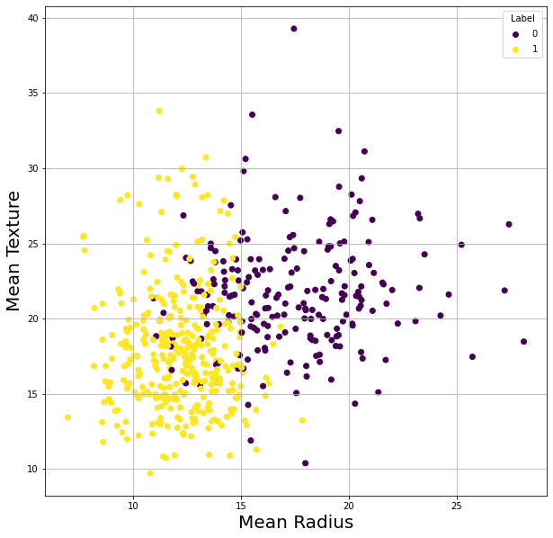
We can use matplotlib to visualize different parts of the dataset
You can find many more plotting examples here: https://colab.research.google.com/notebooks/charts.ipynb
fig, ax = plt.subplots(figsize=[10,10])  #This creates an empty figure of size 10 by 10 inches

#For example we can create a scatter plot of mean radius on the x axis and mean texture on the y axis, and color coded by label
scatter = ax.scatter(df['mean radius'], df['mean texture'], c=df['Label'])
plt.xlabel('Mean Radius', fontsize=20)
plt.ylabel('Mean Texture', fontsize=20)
legend = ax.legend(*scatter.legend_elements(), title="Label") # Note that a label of 0 is malignant and 1 is benign
plt.grid()
plt.show()
4. Basic Analysis
We can use numpy (np) do to some analysis on the data. For example basic descriptive statistics on the tumor features.
We will answer questions such as:
What are the minimum and maximum mean radius in the dataset? What is the mean ‘worst’ smoothness of benign tumors vs malignant tumors?
Feel free to explore other questions
# Minimum and maximum mean radius of all tumors in the dataset:
min_mean_radius = np.min(df['mean radius'])
print('The minimum mean radius is: ', min_mean_radius)

max_mean_radius = np.max(df['mean radius'])
print('The maximum mean radius is: ', max_mean_radius)

# The mean worst smoothness of benign tumors (categorical label equal to 1)
mean_worst_benign_smoothness = np.mean(df.loc[df['Label']==1]['worst smoothness'])  #This selects only cases where tumor is benign (with label equal to 1)
print('The mean worst smoothness of benign tumors is: ', mean_worst_benign_smoothness)

# The mean worst smoothness of malignant tumors (categorical label equal to 1)
mean_worst_malignant_smoothness = np.mean(df.loc[df['Label']==0]['worst smoothness'])  #This selects only cases where tumor is malignant (with label equal to 1)
print('The mean worst smoothness of malignant tumors is: ', mean_worst_malignant_smoothness)
The minimum mean radius is:  6.981
The maximum mean radius is:  28.11
The mean worst smoothness of benign tumors is:  0.12495949579831929
The mean worst smoothness of malignant tumors is:  0.14484523584905656
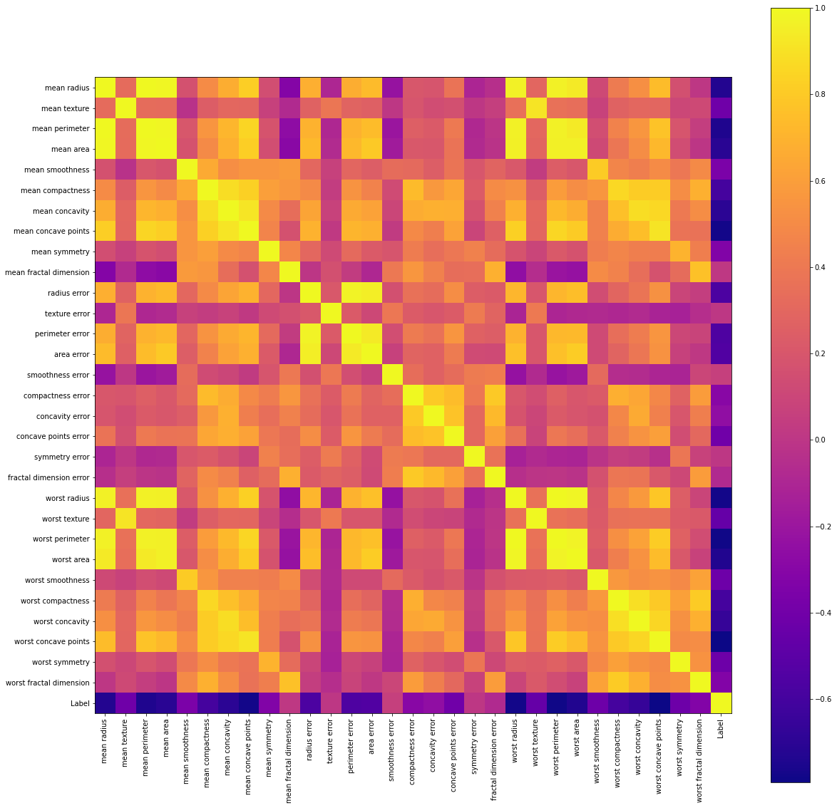
5. More Complex Analysis
In addition to means and ranges of variables, we can explore relationships between variables. For example we can look at the correlation between all variables in the dataset using a simple function on the dataframe, and then visualize it using matplotlib
This makes it easy to visualize which tumor features are well correlated with each other, positively and negatively, and which are not
corr_matrix = df.corr()

fig, ax = plt.subplots(figsize=[20,20])
im = ax.imshow(corr_matrix, cmap='plasma')
ax.set_xticks(np.arange(len(corr_matrix)))
ax.set_yticks(np.arange(len(corr_matrix)))
ax.set_xticklabels(df.columns)
ax.set_yticklabels(df.columns)
plt.xticks(rotation='vertical')
plt.colorbar(im)